";?>
Despite the rather sophisticated derivation, this finally yields a
very elegant scheme that has been implemented in the VMARKET class
FEMSolution.java
as
      double twopi    = 8.*Math.atan(1.);
      double runTime  = runData.getParamValue("RunTime");
      double timeStep = runData.getParamValue("TimeStep");
      double sigma    = runData.getParamValue("Volatility");
      double theta    = runData.getParamValue("TimeTheta");
      double tune     = runData.getParamValue("TuneQuad");
      double lambda   = runData.getParamValue("MktPriceRsk");
      double t        = 1.-time/runTime;               // normalized time
      double hump     = 1.7*(t-t*t*t*t*t*t);           // volatility shaping
      double ca       = runData.getParamValue(runData.meanRevVeloNm);
      double cb       = runData.getParamValue(runData.meanRevTargNm);
      double cycles   = runData.getParamValue(runData.userDoubleNm);
      double cd       = ca*cb-lambda*sigma*Math.cos(twopi*cycles*t);
      double ce       = sigma*hump; ce=ce*ce;
                                                       //--- CONSTRUCT MATRICES
      BandMatrix a = new BandMatrix(3, f.length);      // Linear problem
      BandMatrix b = new BandMatrix(3, f.length);      //  a*fp=b*f=c
      double[]   c = new double[f.length];
                                                       // Quadrature coeff
      double h,h0,h0o,h1,h1m,h1p,h2,h2o;               //  independent of i
      double t0,t0m,t0p,t1,t1m,t1p;                    //  depending on i
      h= dx[0];
      h0o= 0.25*h*(1-tune);               h0= 0.5*h*(1+tune);
      h1m=-0.5; h1p=-h1m;                 h1= 0.;
      h2o=-1./h;                          h2= 2./h;
      for (int i=0; i<=n; i++) {
        t0m=h*h*0.125*(1-tune)*(2*i-1);
        t0p=h*h*0.125*(1-tune)*(2*i+1);   t0=h*h*0.5*i*(tune+1);
        t1m=h*h*0.25*(-2*i-tune+1);
        t1p=h*h*0.25*(-2*i+tune+1);       t1=h*h*0.5*(tune-1);
        a.setL(i,h0o + theta   *timeStep*(t0m +0.5*ce*h2o +ca*t1m +cd*h1m));
        a.setD(i,h0  + theta   *timeStep*(t0  +0.5*ce*h2  +ca*t1  +cd*h1 ));
        a.setR(i,h0o + theta   *timeStep*(t0p +0.5*ce*h2o +ca*t1p +cd*h1p));
        b.setL(i,h0o +(theta-1)*timeStep*(t0m +0.5*ce*h2o +ca*t1m +cd*h1m));
        b.setD(i,h0  +(theta-1)*timeStep*(t0  +0.5*ce*h2  +ca*t1  +cd*h1 ));
        b.setR(i,h0o +(theta-1)*timeStep*(t0p +0.5*ce*h2o +ca*t1p +cd*h1p));
      }
      c=b.dot(f);
      double dPdy0, dPdyn, c0, cn;                     //--- BC
      a.setL(0, 0.);a.setD(0, 1.);a.setR(0, 0.);c[0]=1.;//left: Dirichlet
      double a1n= a.getD(n-1) +4.*a.getL(n-1);         // right: Neuman
      double ann= a.getR(n-1) -3.*a.getL(n-1);         //   O(h^2)
      dPdyn=-time*f[n]; cn=c[n-1]-2*dx[0]*a.getL(n-1)*dPdyn;
      a.setL(n,a1n);a.setD(n,ann);a.setR(n, 0.);c[n]=cn;
      fp=a.solve3(c);                                  //--- SOLVE
      for (int i=0; i<=n; i++) {                       //--- PLOT
        gp[i]=-Math.log(fp[i])/time;                   // yield(r)
        if (time<=timeStep) f0[i]=0.;
      }
      int i=(int)((time/runTime*n));                   // yield(t)
      f0[i]=gp[n/4];
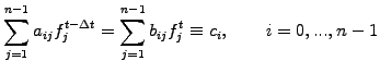
Two band matrices a,b and a vector c are created to first
assemble the linear problem (5.3.1#eq.5) using the commands of the form
a.setL(j,*): they define matrix elements in row  either to the
Left, Right or on the Diagonal of the matrices
either to the
Left, Right or on the Diagonal of the matrices a,b.
The right hand side vector is calculated with a product between the matrix
b and the discount function f that is known from the previous
time step.
The solution fp is computed using
LU factorization
and the
yield is defined from the discount function (2.2.2#eq.1) ready for plotting.
The VMARKET applet below shows the result
obtained for a weakly implicit scheme ( or
or TimeTheta=0.55)
and a tunable integration parameter ( or
or TuneQuad=1.), which
is equivalent to the popular Crank-Nicholson method used by the finite
differences afficinados; to be financially meaningful, the solution has
of course to be independent of the numerical method.
VMARKET applet: press Start/Stop
to study the numerical properties of the finite element implementation
of the Vasicek equation.
Vary the implicit time parameter from explicit to implicit with
TimeTheta in [0.5; 1] and tune the integration TuneQuad
in [0;1] to test a piecewise constant (0) or linear (0.333) FEM
approximation or even a Crank-Nicholson scheme (1).
|
|
"; ?>The finite element formulation is slightly more complicated than the
implicit finite differences but results in the same computational cost.
The additional flexibility provided by a finite elements formulation is
such that the Crank-Nicholson scheme should in fact be of little more
than historical interest.
SYLLABUS Previous: 5.3 Methods for bonds
Up: 5.3 Methods for bonds
Next: 5.3.2 Extensions for derivatives


 ','..','$myPermit') ?>
SYLLABUS Previous: 5.3 Methods for bonds
Up: 5.3 Methods for bonds
Next: 5.3.2 Extensions for derivatives
','..','$myPermit') ?>
SYLLABUS Previous: 5.3 Methods for bonds
Up: 5.3 Methods for bonds
Next: 5.3.2 Extensions for derivatives
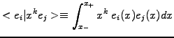
![$\displaystyle \int_{r_-}^{r_+} dr Q \left[ \frac{\partial P}{\partial t} +\frac...
...tial P}{\partial r} - rP \right] = 0 \qquad \forall Q \in \mathcal{C}^1(\Omega)$](s5img91.gif)


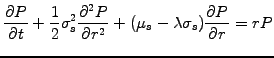
![$\displaystyle \left.
+\bar{\theta}\left(
-\frac{\sigma_s^2}{2} \frac{\partial Q...
...mbda\sigma_s)Q\frac{\partial P^t}{\partial r}\qquad
- rQP^t
\right)
\right]
= 0$](s5img102.gif)
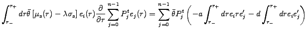
![$\displaystyle \sum_{j=0}^{n-1}
\left[ <e_i \vert e_j>
+\theta\Delta t \left(
\f...
...+ d <e_i \vert e_j^\prime>
+ <e_i \vert re_j>
\right)
\right]P_j^{t-\Delta t} =$](s5img112.gif)
![$\displaystyle \;\sum_{j=0}^{n-1}
\left[ <e_i \vert e_j>
-\bar{\theta}\Delta t \...
... e_j^\prime>
+ d <e_i \vert e_j^\prime>
+ <e_i \vert re_j>
\right)
\right]P_j^t$](s5img113.gif)

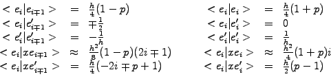
![\begin{displaymath}\left\{
\begin{array}{cl}
(x-x_{j-1})/(x_j-x_{j-1}) \hspace{5...
...m}& x\in[x_j; x_{j+1}]\\
0 & \mathrm{else}
\end{array} \right.\end{displaymath}](s5img134.gif)
![\includegraphics[height=6.5cm]{figs/LinFEM.eps}](s5img136.gif)
![$\displaystyle \int_{x_i}^{x_{i+1}} f(y) dy \approx (x_{i+1}-x_i)\left[\frac{p}{...
...eft[f(x_i)+f(x_{i+1})\right] + (1-p) f\left(\frac{x_i+x_{i+1}}{2}\right)\right]$](s5img137.gif)